How to Design Accurate 5G Networks at 3.5 GHz

Improved coverage and better use of available spectrum are two of the key advantages 5G offers. A properly planned and designed 5G network will support delivery of enhanced mobile broadband applications and experiences, provide more reliable connections for mission-critical communications, and enable the mass deployment of IoT devices.

To capitalize on the benefits 5G offers, the networks that provide coverage indoors must be designed accurately. But planning and designing effective 5G coverage for complex indoor spaces can be much more challenging than existing technologies, like 4G. With so many variables to consider, predicting network performance accurately is the key to deploying a high-quality 5G network end users can rely on.

So, before you tackle any 5G deployment at 3.5 GHz, take a hard look at the prediction software available to support your design process.

An Accurate Network Design Software Eliminates Risk

The accuracy of 5G coverage at 3.5 GHz in any venue is only going to be as good as the software that is used to predict that coverage. Without an accurate software, RF engineers run the risks of delivering a network design that will not perform as needed once it’s installed and activated, and either over-designing or under-designing the network to compensate for variations in the predicted coverage based on wide margins of error.

When a network simulation does not accurately predict how it will perform, once the network is installed, it can lead to very costly troubleshooting, downtime or re-design work. Under-designing the network can create blind spots and negate all the benefits 5G offers. Over-designing the network adds unnecessary equipment costs, complicates deployment and creates more coverage than is needed. Both scenarios can complicate network rollout and add additional costs to a deployment budget.

How can you maximize the accuracy with which you design 5G networks?

You will want to evaluate the features of the software and ensure they are focused on delivering accuracy. Consider:

  • 3D Modeling – If the building is not modeled accurately in the software, then the network simulation will not be accurate either. Ensure that the materials you are modeling with are accurate to the real building, that materials have attenuations set for the frequency you’re designing for, scales are properly set, and all walls and surfaces (including inclined) are included in your model.
  • Accurate Database of Components – The database you are using to model your building and network should contain accurately modeled materials and parts. Ensure the right materials are available and that the parts in the database are accurately modeled vendor parts – antennas, cables, small cells, and other hardware needed for a deployment.
  • Demonstrated accuracy based on stress tests – The software should have a proven history of delivering accurate network simulations and be backed by analytical data and case studies that demonstrate the ability of the software to deliver accurate predictions in a variety of venues, such as stadiums, malls, hotels, and more.
  • Coverage Compliance – The survey tool you use to validate the network should have built in, pre-configured metrics that engineers can use to determine whether design goals have been met, and which network operators can use to verify that the design provided meets all specified goals.

You should also consider different prediction methods and their suitability for particular venues, as not all prediction models have the same accuracy. We’re talking about COST 231, VPLE (Variable Path Loss Equation) and Ray Tracing. You can read more about each and their pros and cons in our dedicated blog.

But of course, the most important consideration is the algorithm the software’s prediction engine uses to generate an accurate prediction.

Accuracy in the prediction process should be based on both mean error and standard deviation.

Mean error is a measure of how much measured data deviates from prediction. If one has collected, say, 400 measured points in a venue, then calculates the difference between predicted and measured value, then sums up the difference in each point and then divides with the number of points, one gets the value for average mean error.

Because the difference in each point can be positive or negative, mean error is sometimes close to zero. But that does not mean that the prediction is very accurate, because the difference in one point could be +20 dB and -20 dB in another, and yet average mean error for those two points is zero.

That’s why it’s very important to also know what the standard deviation should be. This is a number that is always positive and points to how much variation of accuracy can be expected in the prediction.

For inbuilding deployments, the algorithm should be delivering prediction results with a standard deviation and absolute margin of error of 3-5 dB. Anything more than that can lead to an over-designed or under-designed network.

If you want to learn more, read about the 6 Ways iBwave Focuses on Prediction Accuracy.

Deployment Data Confirms Accuracy of Predicted Coverage

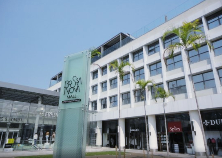
Ultimately, you won’t know how accurate the tool you use is until after you have deployed your network. Data provided by QMC Telecom earlier this year from a 5G trial network at the Bossa Nova Mall in Brazil demonstrates just how important accuracy is when planning in-building coverage.

As outlined in a recent iBwave white paper, the Bossa Nova Mall trial was designed to demonstrate the efficiency of 5G service at 3.5 GHz in indoor environments, so getting optimal coverage in place in high traffic areas was a priority.

After deployment, QMC Telecom compared the predicted and measured 5G coverage. The results show that the accuracy of the prediction tool QMC Telecom used enabled design and deployment of the optimal network configuration to support all trial coverage requirements.

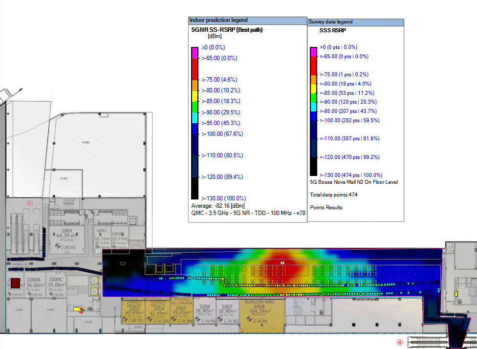
iBwave Design Prediction Accuracy Confirmed at 3.5 GHz

The prediction tool QMC Telecom used was iBwave Design. As the Bossa Nova Mall example shows, iBwave Design provides the right combination of elements needed to streamline the design of all 5G indoor wireless networks, including deployments at 3.5 GHz.

To enable accurate planning and design, the software offers three prediction models — VPLE, COST 231, and Fast Ray Tracing — that provide different levels of accuracy for different environments. Most of our customers rely on the Fast Ray Tracing prediction algorithm, which is based on Ray Tracing and was developed by iBwave RF engineers in partnership with scholars and experts from the in-building industry.

Download the white paper to learn more about how iBwave Design prediction modeling enabled QMC Telecom to accurately design coverage for its 3.5 GHz trial deployment at the Bossa Nova Mall.

___________________________________________

Latest posts by Ali Jemmali (see all)

How Can Machine Learning Help RF Propagation Analysis?

MACHINE LEARNING IN CONTEMPORARY SCIENCE FICTION

2018 movie Annihilation is a science fiction movie about a mysterious area in the southern United States called The Shimmer. The Shimmer started to appear right around the time an identified object from outer space hits a lighthouse near the coastline. Within the Shimmer, rapid species mutation occurs, combining DNA of dissimilar species to make bizarre new species. A team of investigators is sent out to Shimmer, and on their way to the lighthouse they discover and fight grotesque and dangerous mutants.  Once at the lighthouse, the protagonist named Lena (Natalie Portman), squares off against an alien spirit taking form of a threatening big humanoid:

As they start to fight, the humanoid gradually reduces in size, and starts mirroring Lena’s moves:

As the humanoid evolves, it starts to resemble Lena:

Sensing that she is in danger, Lena gives humanoid an incendiary bomb and activates it before running away. The humanoid has never seen an incendiary bomb, and instead of throwing it away it does the only thing it knows what to do: it duplicates the bomb, and throws the copy on the ground:

The humanoid keeps duplicating the bomb in hand, and soon it is engulfed in flames. The fire quickly spreads throughout the lighthouse, burning everything down and destroying the humanoid and the alien spaceship.

The alien humanoid is metaphor for Machine Learning algorithm. For ML to be successful in copying the living organism it needs a lot of data, and that data is Lena’s DNA. ML algorithm also needs time to compute optimum ML coefficients that shape Lena’s body, facial features, and fast track Lena’s moving in real time. However, the ML is not capable of making a good copy of Lena’s memories; when it is given a live incendiary bomb, it cannot rely on memory of Lena’s military training to decide what to do with it. Thus, it makes the wrong decision to copy the bomb instead of getting rid of it.

HOW DOES THIS RELATE TO RF SIGNAL PROPAGATION PREDICTION?

When applied to RF, the ML replicates RF channel between the transmitter (small cell) and the receiver (UE). The input data to ML algorithm can be grouped into 3 data sets:

  1. Transmitter data:
    • Transmitter XYZ coordinates, transmitter power and frequency of operation, transmitter antenna pattern
  2. Environment data:
    • XYZ coordinates, shape and material type of the obstacles between transmitter and receiver
  3. Receiver data
    • UE location XYZ coordinates and RF signal level coverage map, obtained either by
      • RF survey measurements (organic data) or
      • RF simulation software (synthetic data)

Based on the input data, the ML algorithm calculates ML coefficients and recreates RF signal level at UE. The accuracy of ML prediction is compared to the baseline (organic or synthetic data), and ML coefficients are optimized until the prediction error is minimized. Keep in mind that ML propagation algorithm is optimized for specific RF channel, just as the alien spirit optimized the humanoid form for Lena.

What happens when we make a change to input parameters? In general, the ML coefficients need to be recalculated to account for the change. However, some changes are more impactful than others. The change in output power or frequency of operation is not difficult to account for. This is a typical problem for multiband base stations/small cells, as cellular carriers operate at multiple bands. A more difficult problem is to move the transmitter to a different location. A change in the transmitter location changes the environment between the transmitter and UE. An ML algorithm trained on mostly Line of Sight environment would not do well when the small cell is moved to mostly Non-Line of Sight environment. Using an ML algorithm trained on LOS data to predict the NLOS coverage is akin to giving a humanoid a live incendiary bomb. Unlike in the movie there won’t be fireworks and explosions, but the total failure of RF coverage prediction is all but assured.

HOW ACCURATE IS ML PREDICTION?

ML accuracy is always worse than accuracy of the training data. Ideally, we would use only organic RF data to train ML algorithm; however, it is rare that we have enough survey data to do so. Most of the time, we use either synthetic RF data or combination of synthetic and organic training data. Synthetic data is less accurate than organic data, and when trained on synthetic data ML algorithm compounds two errors: the error of synthetic data compared to organic data, and the error of ML data compared to synthetic data. This is a tradeoff when using the ML algorithm for RF prediction; the prediction runs faster but is less accurate.

WHAT IS THE BEST USE FOR ML PREDICTION ALGORITHM?

If one has access to trained ML algorithms for various types of RF channels within a venue, one can simply apply ML algorithm for each transmitter in lieu of Ray Tracing and/or Vector Parabolic Equation simulations. While it takes time to train ML algorithm, reusing appropriate ML is very efficient. Thus, we can greatly reduce computation run time using ML compared to RT/VPE, as the latter must compute RF channel conditions for every transmitter.

The best strategy when designing a large multiband network is to use ML algorithm for preliminary cellular network design, when an RF engineer is still trying to find the optimum transmitter location to maximize the signal coverage. For the final design, the more accurate algorithms (RT/VPE) shall be used for propagation simulation. This methodology still significantly reduces the time to design very large networks, while maintaining the expected accuracy of the final design and final RF coverage maps.

MIMO and Beamforming: Looking at the Impact on Throughput and Coverage

What happens when using MIMO and Beamforming?

A quick brown fox jumps over the lazy dog.

This was a sentence that I heard upward of 500 times when I first started in this business as student intern for a regional mobile wireless carrier. Back then, carriers were transitioning from analog to digital mobile wireless. Aside from signal coverage, the main concern was voice quality of wireless connection. Analog wireless was notorious for garbled and noisy connection, and potential customers were hesitant to buy expensive phones and to pay high “per minute” usage fees to use a product with voice quality vastly inferior to fixed wireless.

To prove that the voice quality is acceptable, we played pre-recorded sentences while on mobile call, and record them on the receiving end while driving around Boulder, CO. Later, the recordings would be played to an impartial audience, which would grade the voice quality. There were about a dozen sentences that we played in a loop; a quick brown fox jumps over the lazy dog is one of those. These days, a chicken leg is a rare dish is another, and rice is often served in round bowls is yet another I still remember. Our test drives would end at the entrance to Boulder Canyon, where the signal would drop.

Let’s see how we can use this sentence to explain what MIMO and Beamforming do to wireless signal throughput and coverage. The setup we used back in the day was basic: one transmit and one receive antenna. Let’s also assume that a modern digital technology would convert the sentence to data, and that it would take one second to transmit that sentence in the basic SISO setup. The coverage edge is the entrance to Boulder Canyon. Now let’s see what happens when use MIMO and Beamforming.

1. MIMO Multiplexing

In this MIMO mode, we split this sentence into 4 parts, and transmit each part on a separate transmit antenna. Those 4 parts are received by 4 receiving antennas and parsed back to its original form. Since each antenna transmits ¼ of the original content, the transmission is completed in 0.25 seconds instead of 1 second. Thus, the transmission rate increased 4 times, while the signal coverage is the same. Technically, due to multipath, each receive antenna may get slightly different signal, and the best of the 4 is selected as receive signal. This is only a slight improvement over the basic SISO setup, which lets us drive about 100 meters into Boulder Canyon before the signal is lost.

Summary: 4 TX, 4Rx antennas, a quick brown fox is 4 times faster, runs 100 meters into Boulder Canyon.

2. MIMO Diversity

In this MIMO mode, each antenna is transmitting the whole sentence. There is no improvement in transmission rate. At the other end, the 4 receive antennas sum the signal up. The resulting signal is higher than what was received at each antenna. As a result, we can hear the sentence even as we drive deeper into Boulder Canyon. The actual net coverage increase is 10*log(4) = 6 dB. This allows us to drive deep into Boulder Canyon before the signal is dropped. Note that we used the number 4 in the equation because there are 4 receive antennas. We would use the same number even if we had only one transmit antenna.

Summary: 4TX, 4RX antennas, a quick brown fox runs one kilometer into Boulder Canyon.

3. Beamforming

Let’s assume that we have 4 transmit antennas and just one receive antenna. This time, we can beamform the transmit antennas. What that means is that we use 4 omnidirectional antenna and make them form a directional antenna pattern if we send signal with slightly different amplitude and phase to each transmit antenna. The directional pattern gain is 10 log(4) = 6 dB higher than individual omnidirectional gain. While it is the same net coverage gain as in the previous case, this time we achieve this coverage improvement with only one receive antenna. While we have slightly more complex network at the base station (signal and phase distribution is different for each antenna), we have fewer antennas at the receiver. Note that the transmission rate is still the same.

Summary: 4TX, 1RX antenna, a quick brown fox runs one kilometer into Boulder Canyon.

4. Beamforming and MIMO

Let’s assume that we have 8 transmit antennas and 2 receive antennas. Half of the transmit and receive antennas have +45° linear polarization, and the other half have -45° polarization. At transmit end, we have 4 collocated +/-45° pairs, and on receive end we have one +/- 45° pair. The four +45° transmit antennas form one directional transmit beam that has 10log(4) = 6dB gain higher than omnidirectional antenna. This beam sends the +45° polarized signal that is recovered by +45° polarized antenna. The same happens with the -45° polarized signal. The original sentence is broken into two halves; one half is sent over +45° polarized signal, and the other half over -45° polarized signal. The whole transmission is completed over 0.5 seconds. Thus, the transmission rate increased 4 times, while the signal increased by 6 dB.

Summary: 8 TX, 2RX antennas, a quick brown fox is 2 times faster, runs one kilometer into Boulder Canyon.

In the next section, we will explain how we configure MIMO streams in iBwave Design.

MIMO Configuration and Beamforming Modeling in iBwave

The first step in considering MIMO configuration in iBwave is to configure the System as MIMO system and for now, there are 4 supported options:

  1. SISO
  2. 2X2 MIMO
  3. 3X3 MIMO
  4. 4X4 MIMO

The number of outputs that can be connected to external antenna will depend on the MIMO configuration:

With MIMO configuration, more than 2 output powers per Path (also called Stream or Branch) and each Path would have its own power. There are three options to connect the output of the systems to the antennas:

  • Use of internal antennas
  • Use of external MIMO antennas (Connect to DAS)
  • Use of external SISO antennas (Connect to DAS)

In iBwave, the output powers (EIRP) of each Path are displayed separately. In the case of an external MIMO antenna or internal antennas, the Output powers of all paths will be displayed in one frame. For the case of external antennas, the Output powers of each antenna will be displayed separately as each antenna can be placed in different location. This concept is shown in the figure below:

The Signal Strength output map is predicted from each path and the strongest value is displayed as a result of prediction. In case of collocated antennas, the predicted values will be almost the same from all paths as they have the same output EIRP power.

As for the MIMO MADR output map, it is predicted for the multiplexing mode and a MIMO Multiplexing Gain is applied from a generic MIMO curve to predict the MADR Throughput map. The Diversity Mode is not supported for now. The MIMO MADR will be the SISO MADR multiplied by the MIMO Gain from the MIMO curve and it is a function of SNR. It is worth noting that the MIMO curve can be configured with specific OEM values.

An example of MIMO gain curve is shown below where the MIMO Gain is a function of SNR

Latest posts by Ali Jemmali (see all)
Exit mobile version