Without a way to generate an accurate prediction of a network design, it can’t be trusted to perform as it’s required to – and when that happens, a lot of time and money is at risk. This is why prediction accuracy has been a focus of iBwave’s since it first started over 16 years ago. It is at the core of what we are focused on and as technologies and learnings have evolved over the years so too has our prediction engine.

Here are the key ways we make sure our prediction is accurate.

1. Fast Ray Tracing

iBwave has three prediction models available in the software: VPLE, COST 231, and Fast Ray Tracing. Each of these prediction methods has different levels of accuracy and are best suited for different environments. At iBwave, because our software is relied upon so often for complex venues, our customers often rely on the Fast Ray Tracing prediction method. This prediction algorithm is based on Ray Tracing and was developed over a period of two years by RF technical experts from iBwave in partnership with scholars and experts from the in-building industry when iBwave first became a company over 16 years ago. But we haven’t stopped developing and improving it along the way – we continue to develop and fine-tune it on an on-going basis to ensure it provides the highest level of accuracy for the venues and technologies modeled in our software.

What is Fast Ray Tracing?

To look at Fast Ray Tracing, let’s first look at COST231. COST231 is the typical algorithm commonly used by other planning software on the market which is an empirical model that only considers a direct path between the transmitter and the receiver. Fast Ray Tracing, on the other hand, considers multiple effects of radio propagation to calculate the signal strength and provide more realistic results. It integrates contributions from direct path (obstructed or not), reflected paths (walls, floors, and ceilings), diffraction and wave guiding effect.

To show this, I’ll take from a previous blog I did that focuses strictly on the impact of considering reflection and diffraction in your predictive designs.

In the following images, I used a highly-reflective warehouse environment and focused on one AP – first with no reflection/diffraction considered and then with reflection/diffraction considered. You see without reflection/ diffraction (image on left) the prediction runs more straight down the warehouse rows. Looking at the prediction considering reflection/diffraction (image on right), you see how the signal reflects and diffracts off the metallic shelves as it travels down the row and gives more coverage to the adjacent rows. Without it, you may over-design the network.

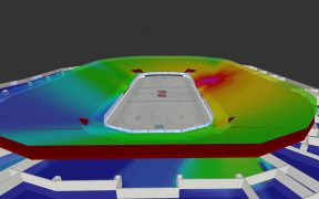
Read: What’s the Impact of Reflection and Diffraction on Prediction Accuracy?

2. Prediction Calibration

If you’ve done a design then you know it can be hard to get an accurate attenuation value for the walls within the venue. And while we’ve put a lot of work into making sure materials in our database are as accurate as possible, in reality, it’s not always accurate. As a result, sometimes an AP on a Stick is used to measure wall loss. But this approach can be both time consuming and does not take into account reflection and diffraction loss. Which is why we have the prediction calibration feature.

With prediction calibration customers have the option to use the measurements taken from a survey to fine-tune the propagation model with live data captured on-site. Essentially what the software does is first try to adjust all propagation parameters and penetration and reflection loss for each material in a floor plan. If for some reason it can’t converge on a solution it will look at all calibrated parameters, choose the least significant one, set it to a default value, and then re-run the calibration without that parameter. This repeats until the solver converges. If the solution has a lot of default settings in the end, it may be a sign that the wrong type of wall material was assigned in the floor plan, or that a wall is missing.

Here is an example of a non-calibrated prediction vs. the survey results

And here is a prediction that has been calibrated using the live survey measurements.

Calibrated Prediction Results vs. Survey

The impact of calibration is obvious in this example: the calibrated prediction comes very close to the survey.

3. Inclined Surfaces

When it comes to certain venues, modeling inclined surfaces, or not, can make a very large difference in prediction results. In the most severe cases this is obvious in a stadium where there is a large number of inclined surfaces to be accounted for. But it can also matter for less complex venues but where inclined surfaces that exist in high-importance areas. For example, the staircase of a hospital where doctors often depend on the wireless network as they move from floor to floor, or the staircase of busy transportation hubs where customers often depend on wireless connectivity.

To highlight the impact it can have, here is the modeling and design of an underground train station that shows the staircase modeled as flat and then the staircase modeled with inclined surfaces. You can see that with the flat model it gives a false impression that some signal strength is present – but when modeled with an inclined surface, you see much of that signal disappear when the prediction is run.

4. Body Loss Modeling

In high-density venues, the attenuation caused by many bodies packed together can make a significant difference. Which is why we have body loss modeling in our software.

Here is a simplified example of the difference it can make. In the first prediction, there is no body loss modeling, and in the second body loss has been modeled for the seating area. In this example, as I probed around the design to compare the values it made a difference of anywhere between 5 to 12 dB difference.

5. 3D Measured Antenna Patterns

When iBwave first launched we used interpolated 2D antenna patterns to get a 3D view in the software. As the years went on and feedback from our customers came indicating that measurements did not match what they saw in the field, we made the change to consider more than just the horizontal and vertical cuts of an antenna pattern. Reaching out to OEMs we asked them to provide measurements for all possible angles for the antenna radiation pattern, which has eliminated the need to do the interpolation from 2D.

Here’s an example of a 3D antenna pattern interpolated from 2D cuts (left) vs. 3D (right) measured and modeled antenna pattern available in iBwave.

And here is an example of the same 2D and 3D antennaes with a 10 degree down tilt aimed at a 30 degree inclined surface.

6. Attenuation by Frequency

We all know that wall attenuation can have a large impact on the accuracy of prediction. In iBwave, the software comes with a large database of various materials with pre-set attenuation values – but the key difference, especially for Wi-Fi, is that it has attenuation values set for all the different frequencies 2.4GHz and 5GHz. And while this may not matter for venues with lighter materials, it can very much matter for environments that use heavier materials such as concrete.

Why does it matter?

If you’ve studied propagation then you already know that as frequency increases, path loss increases. With materials it’s a very similar situation – as frequency increases from 2.4GHz to 5GHz, transmission loss also increases. Imagining a large concrete wall sitting between an AP and a client device, consider that as the 2.4GHz signals move through the wall the attenuation is about 23 dB – now imagine a 5GHz signal moving through the same wall at a higher frequency and you will see the attenuation increase as well to about 45 dB.

In this example, I use concrete as an example with the iBwave default attenuation values set as:

2.4GHz : 22.79
5 GHz: 44.77

You can see the heatmap here that shows signal strength of -81.86 dBm for 5GHz and -55.42 dBM for 2.4GHz

Then I duplicated the material and set the 2.4GHz and 5GHz attenuation values to be the same, using an average attenuation value as the value

2.4GHz: 33.78
5GHz: 33.78

You can see the heatmap here that now shows Signal Strength of -70.09 for 5GHz and -65.53 for 2.4GHz

In this case, having different attenuation values makes a fairly significant difference in prediction results.

That’s a Wrap.

While there are many other factors in how accurate a prediction is for any given design (for example the model itself), these are just six of the many ways that iBwave works to achieve the most accurate prediction accuracy.

Hope you enjoyed the blog and see you next time!

Accurately yours,

Kelly

Depending on the venue you’re designing, considering reflection and diffraction can make anywhere from a small to a very large difference. Take a small open office space for example – reflection and diffraction probably don’t make such a large difference. But when you look at more complex venues such as a warehouse, or large manufacturing facility full of metal shelves, machinery and inventory? You’re going to see a much larger difference.

To dive deeper into what this looks like and the impact it can have, I took an example warehouse modeled with inventory shelves and boxes and predicted network performance in two ways:

Considering both reflection and diffraction in the prediction results (the default in iBwave)
Without reflection and diffraction in the prediction results

By running these two scenarios, I could see the impact considering reflection/diffraction in prediction vs. just looking at direct path can have on a design. I did this both for the overall design and then later one just looking at one access point in isolation.

About the Venue and Design

The venue I used is a demo warehouse that has been modeled with offices, metal shelves with stacked inventory boxes, and the then the usual walls and metal roof structure of a typical large warehouse venue. In terms of the Wi-Fi network design, there are a total of 14 APs placed with antennas. Details can be seen on the Bill of Materials report.

In 3D the warehouse model looks like this ?

Prediction Results: With Reflection & Diffraction Considered

The first scenario I wanted to look at was the default scenario in iBwave where both reflection and diffraction of the wireless signals are considered as they move through the warehouse space and objects – this is done using the Fast Ray Tracing prediction method, the most accurate of the three available (others include VPLE, and COST231) . It’s essentially what would be considered the most accurate prediction simulation.

Looking at the Signal Strength heatmap for 2.4GHz you see the coverage of the warehouse floor.

And in 3D…

Prediction Results: No Reflection & Diffraction Considered

Next, I went into the output map configuration options and removed the option to consider reflection and diffraction from the prediction algorithm to see what the impact would be on the simulation of the network performance. (Note: this feature is only available for internal debugging purposes and is not in the general release of the software.)

Then I ran the 2.4GHz Signal Strength heatmap again to see what the difference in results were compared to when the algorithm considered reflection/diffraction. You can see just from the heatmap visual alone there is a difference, where because reflection and diffraction are not considered, the prediction considers only direct path and as a result shows more areas of weak signal (blue).

Taking a Closer Look at the Difference

Now that we’ve simulated both scenarios – with reflection/diffraction versus without – we can examine the difference between the two closer using two different ways:

By using the heatmap probe to closer examine the result of the heatmaps in specific spots
Generate a ‘Subtraction Heatmap’ which will show the performance difference between the two heatmaps – basically results with reflection vs. results without.

Using the Subtraction Heatmap

First let’s look at the Subtraction Heatmap which gives us an overall view of what the difference is between the heatmaps that consider reflection/diffraction, and the heatmap that does not.

Considering a difference of +/- 3dBM as acceptable, you can see that while the majority of the heatmap falls into this category (green), there are some rather large areas (purple) that fall into an unacceptable range ( > 3 dBM and up to 30 dBM).

Using the Heatmap Probe

Now using the probe tool on the heatmap, we can mouse over specific spots and get a comparison reading for the ‘With Reflection/Diffraction’ heatmap versus the ‘Without Reflection/Diffraction’ heatmap. By doing this, we can see a difference of up to 30 dBm in some areas, and in this particular spot it is a significant difference of -24.70 dBm.

Looking at an Example in Isolation

Next, I wanted to just isolate one access point and run prediction with/without reflection and diffraction considered to see the impact from an isolated perspective.

Here are the results when reflection and diffraction are considered in the prediction algorithm. Using the 3D view of the heatmap, you can see how the signal coming out from the AP reflects and diffracts as they meet the shelves and inventory of the warehouse.

When you remove the reflection and diffraction from the prediction algorithm, you see how only the direct path is considered, giving a very straight pathway down the inventory shelves in the warehouse. Again, the 3D view helps us visualize that impact pretty easily, especially towards the end of the inventory row where you see no reflection/diffraction off the objects in the path.

What’s the Impact?

Given the large difference in prediction results when looking at this example of a warehouse, it becomes obvious that considering reflection and diffraction within the prediction results can have a significant impact on the accuracy of the network performance simulation. In this case, without considering it, the network designer may add more APs where weak signal zones appear because only direct path is considered in the simulation. As a result, the network may be over-designed leading to more cost and issues that require troubleshooting once the network is installed and turned on.

In a more open floor plan, reflection and diffraction probably would not have such a large impact. But in environments where there is a lot of metal and obstacles (warehouse being a great example) , considering the impact of reflection and diffraction in the prediction algorithm has a significant impact on the accuracy of your network simulation, and design.

Wirelessly yours,