
6 Ways iBwave Focuses on Prediction Accuracy
Share
Without a way to generate an accurate prediction of a network design, it can’t be trusted to perform as it’s required to – and when that happens, a lot of time and money is at risk. This is why prediction accuracy has been a focus of iBwave’s since it first started over 16 years ago. It is at the core of what we are focused on and as technologies and learnings have evolved over the years so too has our prediction engine.
Here are the key ways we make sure our prediction is accurate.
1. Fast Ray Tracing
iBwave has three prediction models available in the software: VPLE, COST 231, and Fast Ray Tracing. Each of these prediction methods has different levels of accuracy and are best suited for different environments. At iBwave, because our software is relied upon so often for complex venues, our customers often rely on the Fast Ray Tracing prediction method. This prediction algorithm is based on Ray Tracing and was developed over a period of two years by RF technical experts from iBwave in partnership with scholars and experts from the in-building industry when iBwave first became a company over 16 years ago. But we haven’t stopped developing and improving it along the way – we continue to develop and fine-tune it on an on-going basis to ensure it provides the highest level of accuracy for the venues and technologies modeled in our software.
What is Fast Ray Tracing?
To look at Fast Ray Tracing, let’s first look at COST231. COST231 is the typical algorithm commonly used by other planning software on the market which is an empirical model that only considers a direct path between the transmitter and the receiver. Fast Ray Tracing, on the other hand, considers multiple effects of radio propagation to calculate the signal strength and provide more realistic results. It integrates contributions from direct path (obstructed or not), reflected paths (walls, floors, and ceilings), diffraction and wave guiding effect.
To show this, I’ll take from a previous blog I did that focuses strictly on the impact of considering reflection and diffraction in your predictive designs.
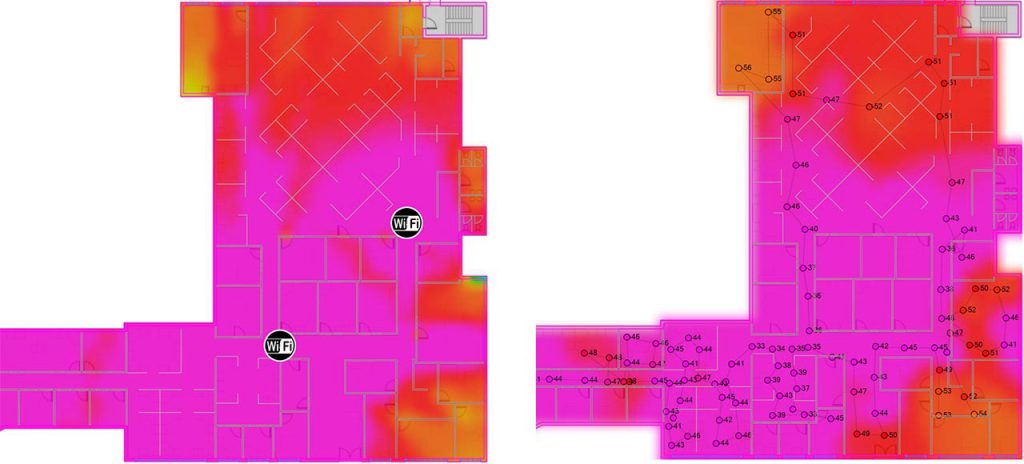
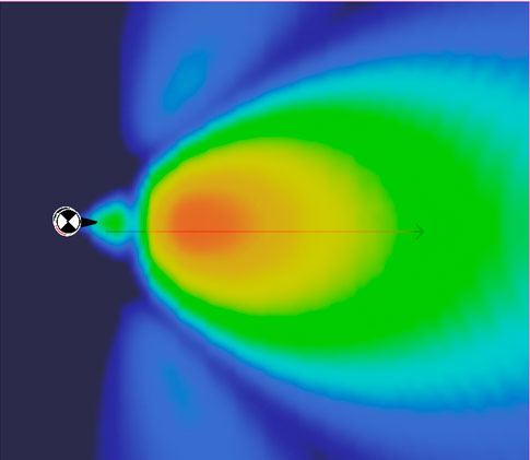
In the following images, I used a highly-reflective warehouse environment and focused on one AP – first with no reflection/diffraction considered and then with reflection/diffraction considered. You see without reflection/ diffraction (image on left) the prediction runs more straight down the warehouse rows. Looking at the prediction considering reflection/diffraction (image on right), you see how the signal reflects and diffracts off the metallic shelves as it travels down the row and gives more coverage to the adjacent rows. Without it, you may over-design the network.
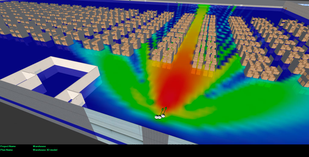
No Reflection or Diffraction 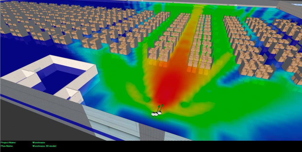
With Reflection and Diffraction
Read: What’s the Impact of Reflection and Diffraction on Prediction Accuracy?
2. Prediction Calibration
If you’ve done a design then you know it can be hard to get an accurate attenuation value for the walls within the venue. And while we’ve put a lot of work into making sure materials in our database are as accurate as possible, in reality, it’s not always accurate. As a result, sometimes an AP on a Stick is used to measure wall loss. But this approach can be both time consuming and does not take into account reflection and diffraction loss. Which is why we have the prediction calibration feature.
With prediction calibration customers have the option to use the measurements taken from a survey to fine-tune the propagation model with live data captured on-site. Essentially what the software does is first try to adjust all propagation parameters and penetration and reflection loss for each material in a floor plan. If for some reason it can’t converge on a solution it will look at all calibrated parameters, choose the least significant one, set it to a default value, and then re-run the calibration without that parameter. This repeats until the solver converges. If the solution has a lot of default settings in the end, it may be a sign that the wrong type of wall material was assigned in the floor plan, or that a wall is missing.
Here is an example of a non-calibrated prediction vs. the survey results
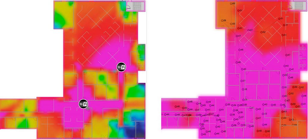
And here is a prediction that has been calibrated using the live survey measurements.
The impact of calibration is obvious in this example: the calibrated prediction comes very close to the survey.
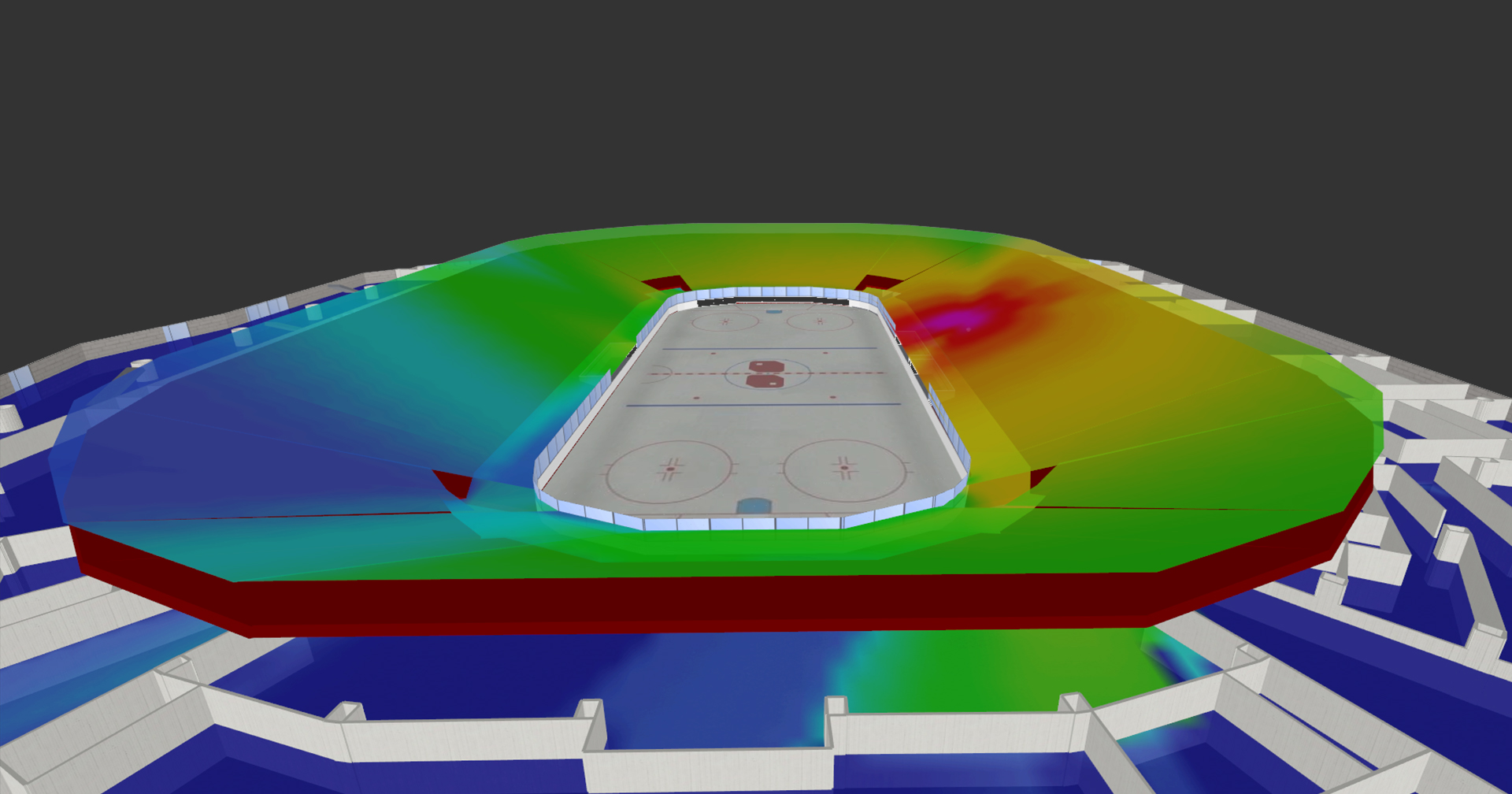
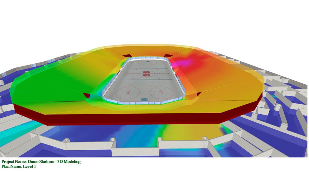
3. Inclined Surfaces
When it comes to certain venues, modeling inclined surfaces, or not, can make a very large difference in prediction results. In the most severe cases this is obvious in a stadium where there is a large number of inclined surfaces to be accounted for. But it can also matter for less complex venues but where inclined surfaces that exist in high-importance areas. For example, the staircase of a hospital where doctors often depend on the wireless network as they move from floor to floor, or the staircase of busy transportation hubs where customers often depend on wireless connectivity.
To highlight the impact it can have, here is the modeling and design of an underground train station that shows the staircase modeled as flat and then the staircase modeled with inclined surfaces. You can see that with the flat model it gives a false impression that some signal strength is present – but when modeled with an inclined surface, you see much of that signal disappear when the prediction is run.
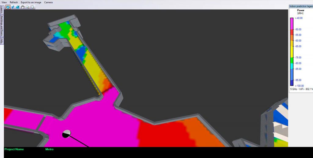
No Inclined Modeled 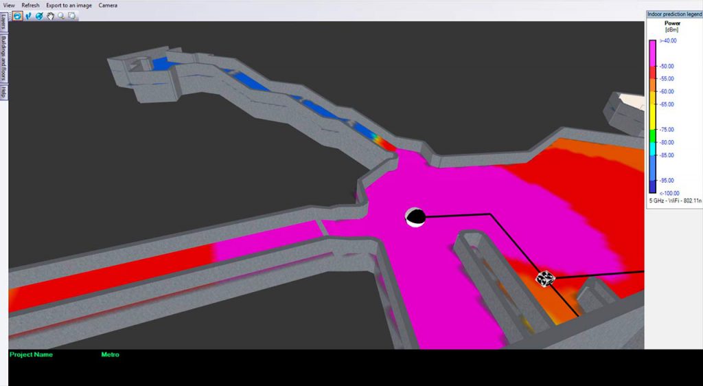
Inclined Modeled
4. Body Loss Modeling
In high-density venues, the attenuation caused by many bodies packed together can make a significant difference. Which is why we have body loss modeling in our software.
Here is a simplified example of the difference it can make. In the first prediction, there is no body loss modeling, and in the second body loss has been modeled for the seating area. In this example, as I probed around the design to compare the values it made a difference of anywhere between 5 to 12 dB difference.
No Body Loss Modeled 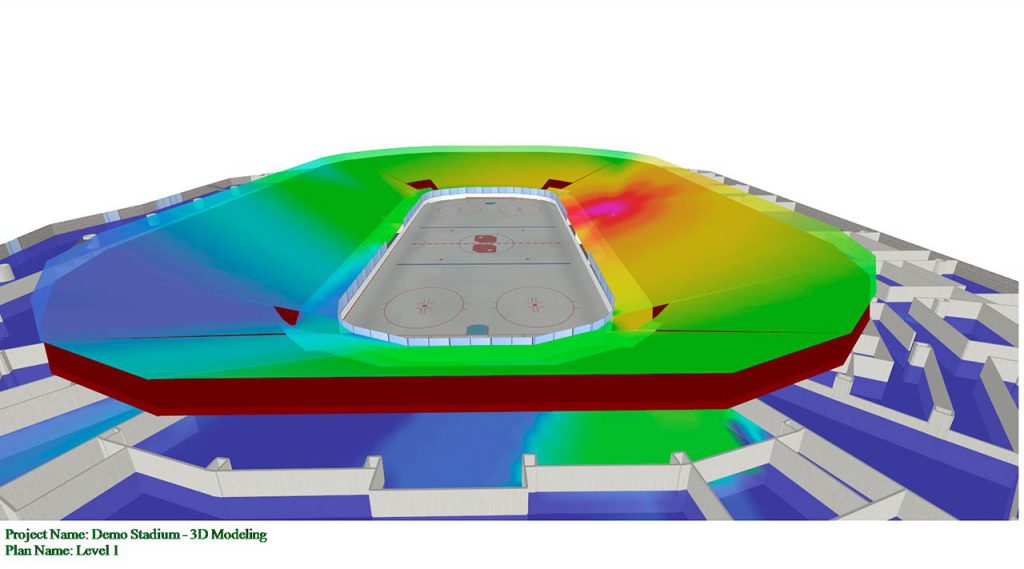
Body Loss Modeled
5. 3D Measured Antenna Patterns
When iBwave first launched we used interpolated 2D antenna patterns to get a 3D view in the software. As the years went on and feedback from our customers came indicating that measurements did not match what they saw in the field, we made the change to consider more than just the horizontal and vertical cuts of an antenna pattern. Reaching out to OEMs we asked them to provide measurements for all possible angles for the antenna radiation pattern, which has eliminated the need to do the interpolation from 2D.
Here’s an example of a 3D antenna pattern interpolated from 2D cuts (left) vs. 3D (right) measured and modeled antenna pattern available in iBwave.
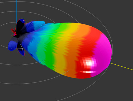
2D Interpolated Antenna Pattern 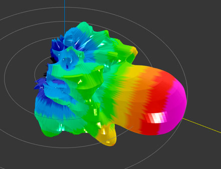
3D Measured Antenna Pattern
And here is an example of the same 2D and 3D antennaes with a 10 degree down tilt aimed at a 30 degree inclined surface.
2D Interpolated (2.4GHz) 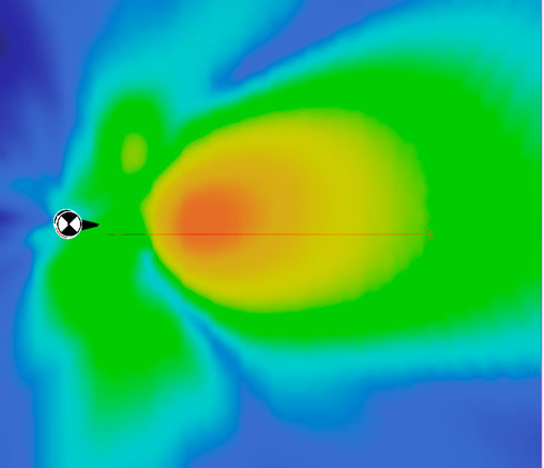
3D Measured (2.4GHz)
6. Attenuation by Frequency
We all know that wall attenuation can have a large impact on the accuracy of prediction. In iBwave, the software comes with a large database of various materials with pre-set attenuation values – but the key difference, especially for Wi-Fi, is that it has attenuation values set for all the different frequencies 2.4GHz and 5GHz. And while this may not matter for venues with lighter materials, it can very much matter for environments that use heavier materials such as concrete.
Why does it matter?
If you’ve studied propagation then you already know that as frequency increases, path loss increases. With materials it’s a very similar situation – as frequency increases from 2.4GHz to 5GHz, transmission loss also increases. Imagining a large concrete wall sitting between an AP and a client device, consider that as the 2.4GHz signals move through the wall the attenuation is about 23 dB – now imagine a 5GHz signal moving through the same wall at a higher frequency and you will see the attenuation increase as well to about 45 dB.
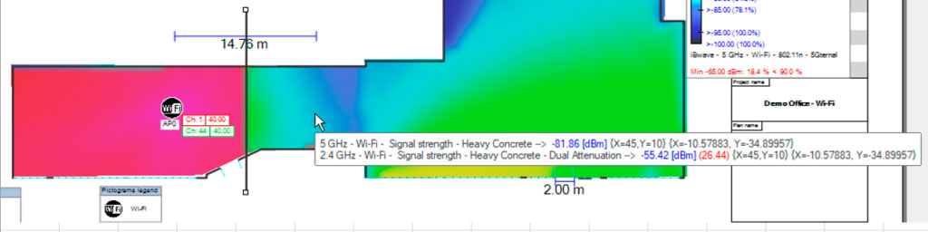
In this example, I use concrete as an example with the iBwave default attenuation values set as:
- 2.4GHz : 22.79
- 5 GHz: 44.77
You can see the heatmap here that shows signal strength of -81.86 dBm for 5GHz and -55.42 dBM for 2.4GHz
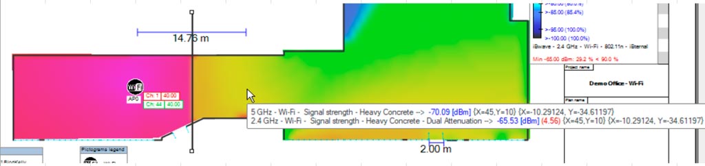
Then I duplicated the material and set the 2.4GHz and 5GHz attenuation values to be the same, using an average attenuation value as the value
- 2.4GHz: 33.78
- 5GHz: 33.78
You can see the heatmap here that now shows Signal Strength of -70.09 for 5GHz and -65.53 for 2.4GHz
In this case, having different attenuation values makes a fairly significant difference in prediction results.
That’s a Wrap.
While there are many other factors in how accurate a prediction is for any given design (for example the model itself), these are just six of the many ways that iBwave works to achieve the most accurate prediction accuracy.
Hope you enjoyed the blog and see you next time!
Accurately yours,
Kelly
Kelly Burroughs has worked in the wireless industry over the last 8 years in a variety of roles. Her background in product, marketing, and wireless jokes makes her a triple threat in the industry. When she’s not busy trying to improve the wireless survey & design experience for customers, she can be found writing wireless jokes that make even the most dedicated network engineer smile (or roll their eyes).
- The Enterprise Guide to Better Cellular Connectivity - June 11, 2026
- Cleared for Takeoff: Private Networks in Aviation - January 21, 2025
- A Tour of iBwave Viewer - November 23, 2020


Excellent explanation, thanks a lot.