
Category: Enterprises

Earth Day is a time to commemorate the importance of respecting the environment and making changes towards a greener future. This year we are emphasizing the importance of e-waste. As a team, at iBwave, we worked together in collecting e-waste from our homes and offices to dispose of properly. What is E-Waste? E-waste (electronic waste) […]
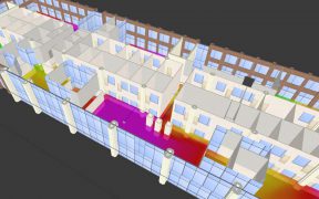
Available for many years and compatible with all our software, iBwave’s free read-only viewer is a popular go-to for the customers of our customers to review survey and design work done on their projects. In this blog I’ll take you on a quick tour of what it can do. An Overview of iBwave Viewer Features […]

Some of you already know we’ve been playing with the idea of how to use Augmented Reality in the wireless network design process for the last little while. It’s been a fun innovation project to work on and a fun one to show people along the way at various conferences and events. But we wanted […]