
MIMO and Beamforming: Looking at the Impact on Throughput and Coverage
Share

What happens when using MIMO and Beamforming?
A quick brown fox jumps over the lazy dog.
This was a sentence that I heard upward of 500 times when I first started in this business as student intern for a regional mobile wireless carrier. Back then, carriers were transitioning from analog to digital mobile wireless. Aside from signal coverage, the main concern was voice quality of wireless connection. Analog wireless was notorious for garbled and noisy connection, and potential customers were hesitant to buy expensive phones and to pay high “per minute” usage fees to use a product with voice quality vastly inferior to fixed wireless.
To prove that the voice quality is acceptable, we played pre-recorded sentences while on mobile call, and record them on the receiving end while driving around Boulder, CO. Later, the recordings would be played to an impartial audience, which would grade the voice quality. There were about a dozen sentences that we played in a loop; a quick brown fox jumps over the lazy dog is one of those. These days, a chicken leg is a rare dish is another, and rice is often served in round bowls is yet another I still remember. Our test drives would end at the entrance to Boulder Canyon, where the signal would drop.
Let’s see how we can use this sentence to explain what MIMO and Beamforming do to wireless signal throughput and coverage. The setup we used back in the day was basic: one transmit and one receive antenna. Let’s also assume that a modern digital technology would convert the sentence to data, and that it would take one second to transmit that sentence in the basic SISO setup. The coverage edge is the entrance to Boulder Canyon. Now let’s see what happens when use MIMO and Beamforming.
1. MIMO Multiplexing
In this MIMO mode, we split this sentence into 4 parts, and transmit each part on a separate transmit antenna. Those 4 parts are received by 4 receiving antennas and parsed back to its original form. Since each antenna transmits ¼ of the original content, the transmission is completed in 0.25 seconds instead of 1 second. Thus, the transmission rate increased 4 times, while the signal coverage is the same. Technically, due to multipath, each receive antenna may get slightly different signal, and the best of the 4 is selected as receive signal. This is only a slight improvement over the basic SISO setup, which lets us drive about 100 meters into Boulder Canyon before the signal is lost.
Summary: 4 TX, 4Rx antennas, a quick brown fox is 4 times faster, runs 100 meters into Boulder Canyon.
2. MIMO Diversity
In this MIMO mode, each antenna is transmitting the whole sentence. There is no improvement in transmission rate. At the other end, the 4 receive antennas sum the signal up. The resulting signal is higher than what was received at each antenna. As a result, we can hear the sentence even as we drive deeper into Boulder Canyon. The actual net coverage increase is 10*log(4) = 6 dB. This allows us to drive deep into Boulder Canyon before the signal is dropped. Note that we used the number 4 in the equation because there are 4 receive antennas. We would use the same number even if we had only one transmit antenna.
Summary: 4TX, 4RX antennas, a quick brown fox runs one kilometer into Boulder Canyon.
3. Beamforming
Let’s assume that we have 4 transmit antennas and just one receive antenna. This time, we can beamform the transmit antennas. What that means is that we use 4 omnidirectional antenna and make them form a directional antenna pattern if we send signal with slightly different amplitude and phase to each transmit antenna. The directional pattern gain is 10 log(4) = 6 dB higher than individual omnidirectional gain. While it is the same net coverage gain as in the previous case, this time we achieve this coverage improvement with only one receive antenna. While we have slightly more complex network at the base station (signal and phase distribution is different for each antenna), we have fewer antennas at the receiver. Note that the transmission rate is still the same.
Summary: 4TX, 1RX antenna, a quick brown fox runs one kilometer into Boulder Canyon.
4. Beamforming and MIMO
Let’s assume that we have 8 transmit antennas and 2 receive antennas. Half of the transmit and receive antennas have +45° linear polarization, and the other half have -45° polarization. At transmit end, we have 4 collocated +/-45° pairs, and on receive end we have one +/- 45° pair. The four +45° transmit antennas form one directional transmit beam that has 10log(4) = 6dB gain higher than omnidirectional antenna. This beam sends the +45° polarized signal that is recovered by +45° polarized antenna. The same happens with the -45° polarized signal. The original sentence is broken into two halves; one half is sent over +45° polarized signal, and the other half over -45° polarized signal. The whole transmission is completed over 0.5 seconds. Thus, the transmission rate increased 4 times, while the signal increased by 6 dB.
Summary: 8 TX, 2RX antennas, a quick brown fox is 2 times faster, runs one kilometer into Boulder Canyon.
In the next section, we will explain how we configure MIMO streams in iBwave Design.
MIMO Configuration and Beamforming Modeling in iBwave
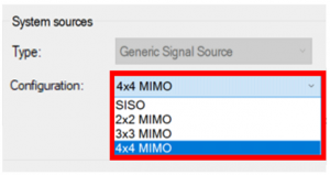
The first step in considering MIMO configuration in iBwave is to configure the System as MIMO system and for now, there are 4 supported options:
- SISO
- 2X2 MIMO
- 3X3 MIMO
- 4X4 MIMO
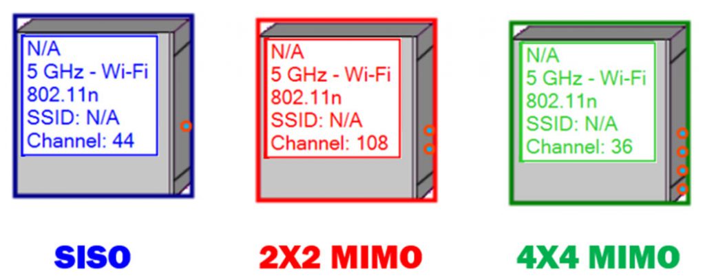
The number of outputs that can be connected to external antenna will depend on the MIMO configuration:
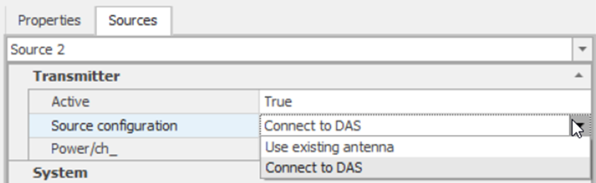
With MIMO configuration, more than 2 output powers per Path (also called Stream or Branch) and each Path would have its own power. There are three options to connect the output of the systems to the antennas:
- Use of internal antennas
- Use of external MIMO antennas (Connect to DAS)
- Use of external SISO antennas (Connect to DAS)
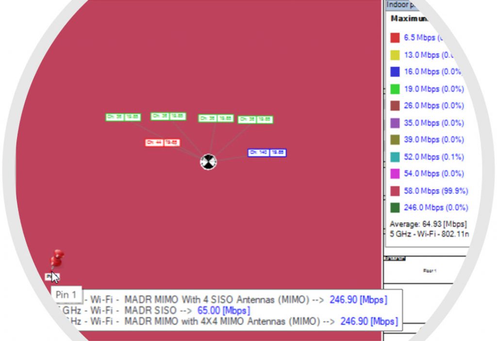
In iBwave, the output powers (EIRP) of each Path are displayed separately. In the case of an external MIMO antenna or internal antennas, the Output powers of all paths will be displayed in one frame. For the case of external antennas, the Output powers of each antenna will be displayed separately as each antenna can be placed in different location. This concept is shown in the figure below:
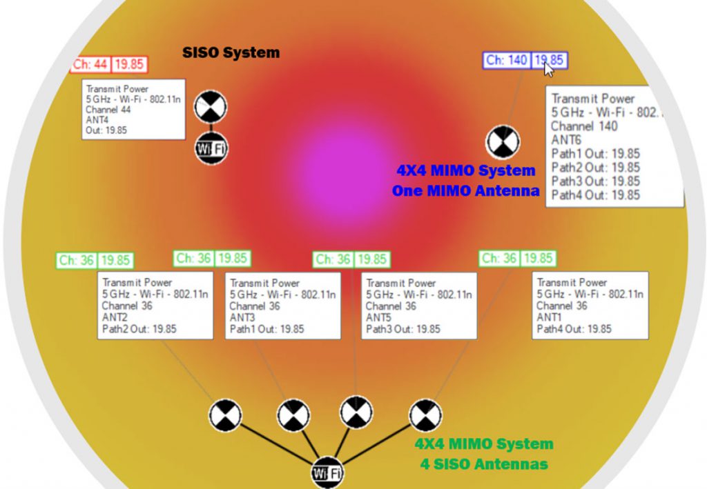
The Signal Strength output map is predicted from each path and the strongest value is displayed as a result of prediction. In case of collocated antennas, the predicted values will be almost the same from all paths as they have the same output EIRP power.
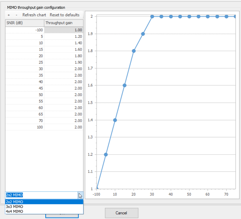
As for the MIMO MADR output map, it is predicted for the multiplexing mode and a MIMO Multiplexing Gain is applied from a generic MIMO curve to predict the MADR Throughput map. The Diversity Mode is not supported for now. The MIMO MADR will be the SISO MADR multiplied by the MIMO Gain from the MIMO curve and it is a function of SNR. It is worth noting that the MIMO curve can be configured with specific OEM values.
An example of MIMO gain curve is shown below where the MIMO Gain is a function of SNR
Vladan Jevremovic joined iBwave in 2009 as director of Engineering Solutions and has been in the Telecommunication industry for more than 17 years. He is responsible for developing custom solutions as a part of a professional services portfolio. He’s also responsible for ideation and requirements specification in the new product development life cycle, and works closely with the development team on new product implementation. Vladan received his Diploma Ing. from the University of Belgrade in Serbia, and his Masters and Ph.D. from the University of Colorado Boulder.
- Private: How to Design Accurate 5G Networks at 3.5 GHz – November 23, 2022
- How Can Machine Learning Help RF Propagation Analysis? – November 19, 2021
- MIMO and Beamforming: Looking at the Impact on Throughput and Coverage – April 27, 2021
Ali Jemmali is an experienced research and development specialist with a demonstrated history of working in the wireless industry. He is skilled in MIMO, Wideband Code Division Multiple Access (WCDMA), LTE, 4G, and RF Planning. He is a strong media and communication professional with a Doctor of Philosophy (Ph.D.) focused in Electrical Engineering from Université de Montréal – École Polytechnique de Montréal.
- Private: Power Output & MIMO – Predictive Design – April 23, 2021
Vladan Jevremovic has joined iBwave in 2009 as Director of Engineering Solutions and has been in the Telecommunication industry for more than 17 years. He is responsible for developing custom solutions as a part of professional services portfolio. He’s also responsible for ideation and requirements specification in the new product development life cycle, and works closely with the development team on new product implementation. Vladan received his Diploma Ing. from University of Belgrade in Serbia, and his Masters and PhD from University of Colorado at Boulder.
- A Deep Dive into iBwave Design Prediction Accuracy Report - November 18, 2024
- At a Glance: What Is New in Wi-Fi 7? - July 4, 2024
- Accurate Prediction Simplifies Private, In-Building 5G Network Deployments - March 1, 2023


